Once you have any GeolOil license (even a non-commercial license), you may acquire our server access service to an extra data set examples of fully interpreted well logs. The server access will last until the life term of your license.

Even if you regularly use another commercial petrophysical software, it is a hands-on valuable tool to understand petrophysical concepts, interpretation and computation work-flows. Learn how to compute porosity from different sources, matrix density, rock strength, shaliness, mineral proportions solvers, scripting, and produce nice log displays. The data collection occasionally grows with key cases from naturally fractured reservoirs, clastic reservoirs, carbonate reservoirs, unconventional tight, and shale oil reservoirs.

     

Following down is a selection of some relevant processed log examples, that ships out of the box with the Learn Set:

---

• A geomechanics study to assess a reservoir cap rock integrity against induced fractures by injection pressure.
  
  ✔ GLOG File: BoreHoleStability_web.glog
  
  An injection process is carried out into an eolian gas reservoir. While in this particular operational case, does not matter if the reservoir zone can become fractured, it is required that the anhydrite cap rock can resist the injection and no fractures would be induced. Cap rock integrity is essential to avoid leaks in environmental problems, and contain pressure.
  The anhydrite cap rock studied is strong and ductile enough to avoid the creation of fractures. In all sensibility scenarios of rock strength and a window of three injection pressures, a competent continuous anhydrite cap rock of a least 13' was found, enough to avoid fractures and fulfill government environmental regulations. See the log plot below ↓

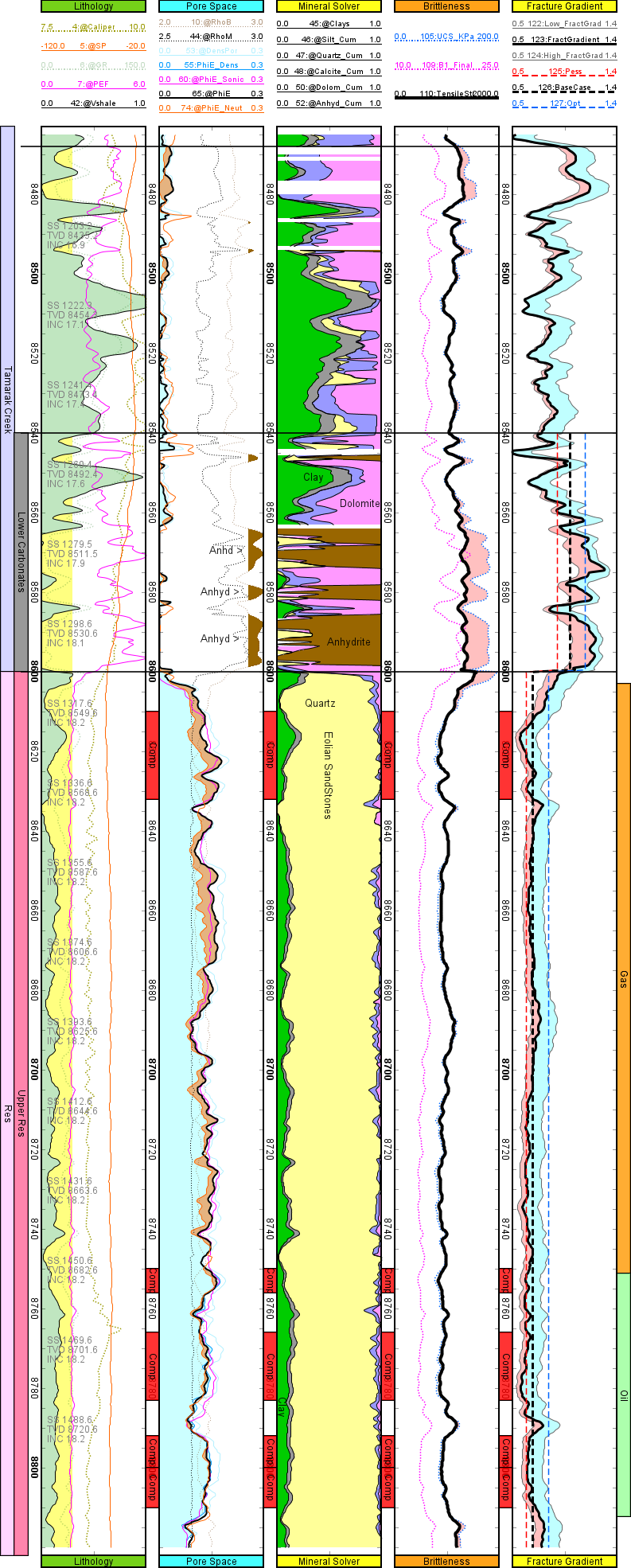
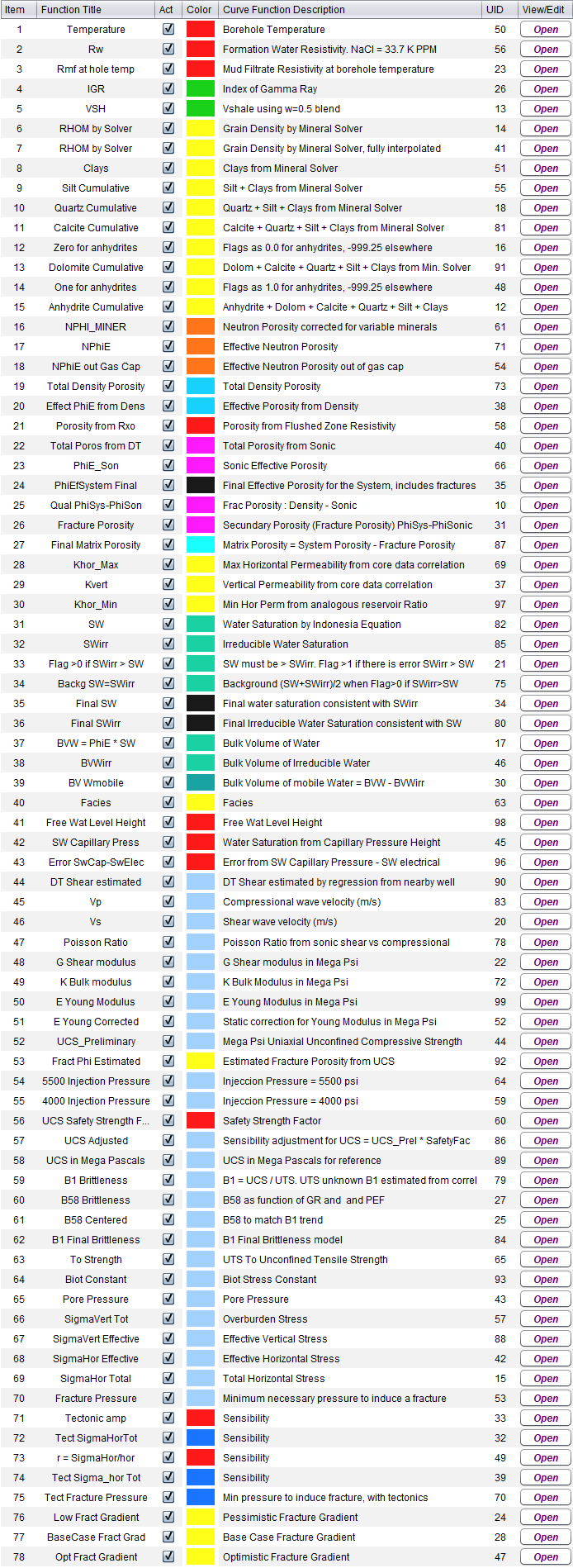
The functions panel work-flow below details all the functions and equations used, including an essential petrophysical study with a carbonate mineral solver, estimations of rock brittleness and strength, geomechanical stresses, and fracture gradients. The use of a mineral solver was essential in this study as it detected that the cap rock is an anhydrite, which is very strong and has its own geomechanical properties:

---

• How to do a variable depth shift of curves on a LAS log file.
  
  ✔ GLOG File: variable_shift_example.glog
  
  GeolOil has three methods to process depth shifts on log curves: 1) Manually, using the matrix table editor tab, 2) By built-in functions in the work-flow tab, and 3) By using a very small script with GeolOil GLS. A case example is provided with plenty of details in the log plot below ↓

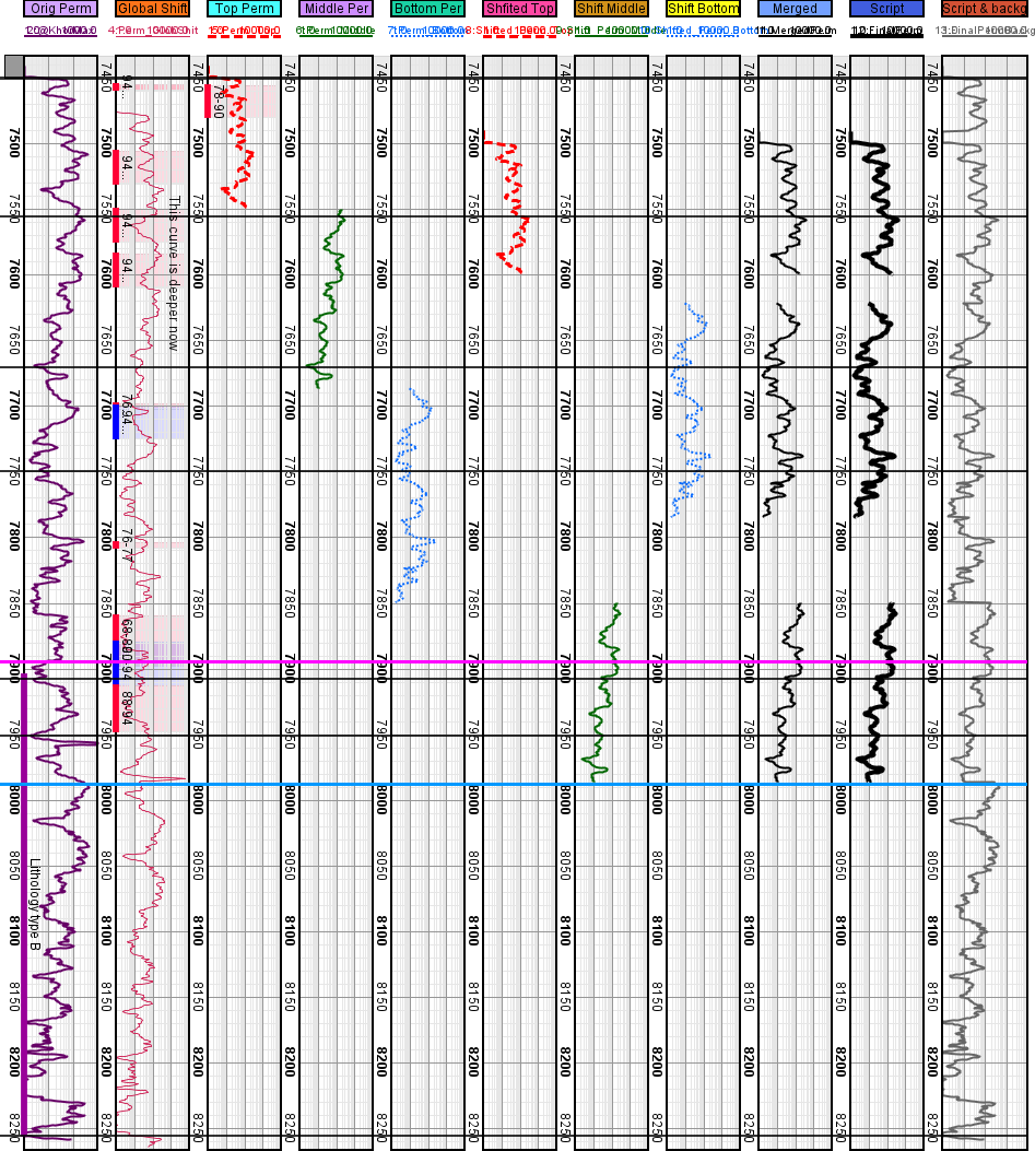
The functions panel work-flow below shows all the functions and a small script used:

---

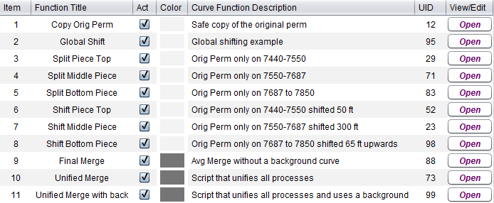
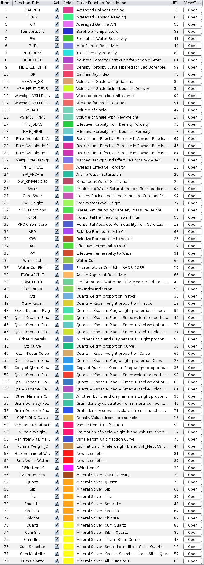
• A clastic braided channels reservoir with a clay mineral solver.
  
  ✔ GLOG File: claySolver.glog
  
  This example shows how estimate the major different clay minerals of a clastic reservoir. The last two log tracks display the clay composition through the semi-quantitative technique of X-Ray diffraction, and the solution found by the GeolOil clay mineral solver. Clay discrimination is always difficult. However the mineral solved estimations, show a reasonable qualitative match against the X-Ray diffraction reference track.
  
  The most dominant found clay is smectite. However, around the depth MD=1820 ft., the mineral solver correctly detected the presence of the clay mineral kaolinte, which is particularly difficult to detect as its Gamma Ray response is usually low due to its low Cation Exchange Capacity. Notice on the first Lithology track, how low is the GR Gamma Ray signal compared with signal yielded by a neutron porosity minus density porosity estimator VSH. See the log plot below ↓

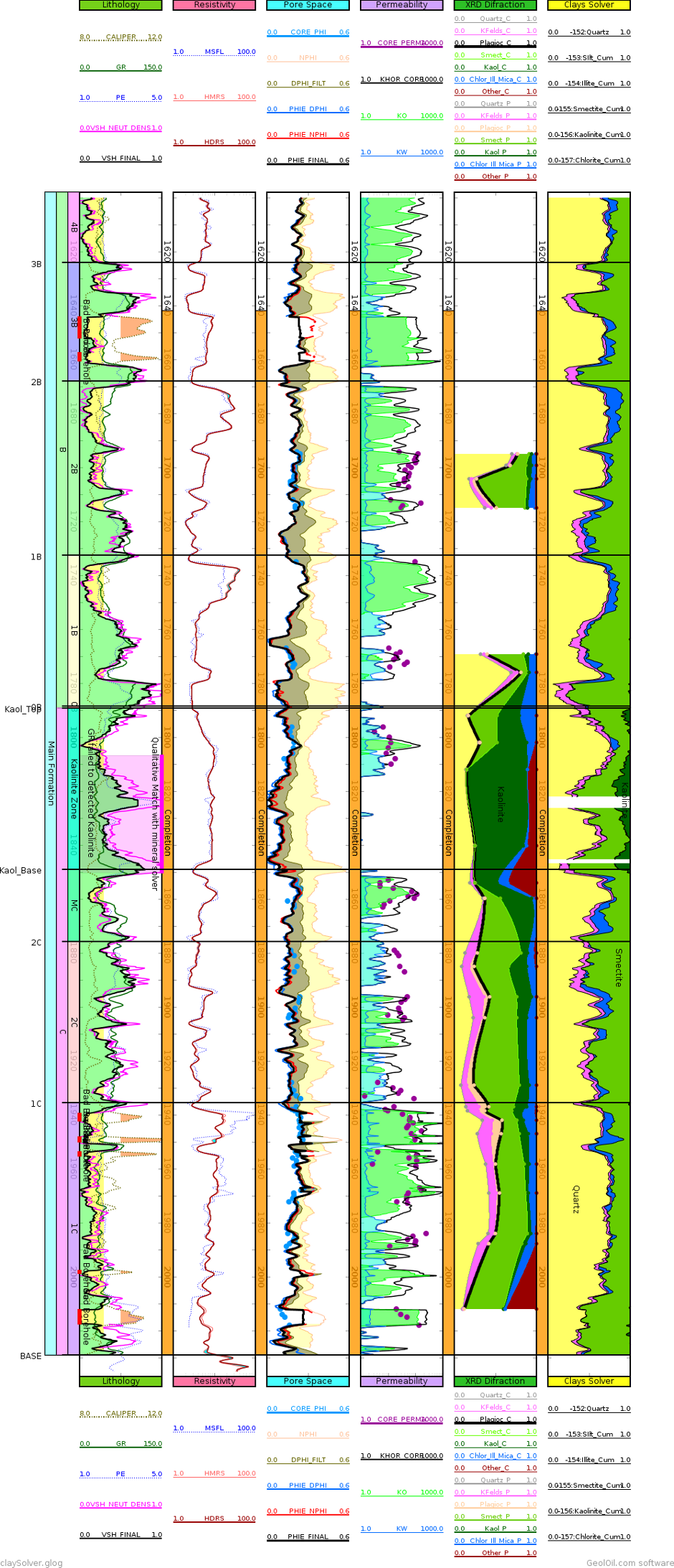
The functions panel work-flow below shows all the functions and equations used, including the volume of shale VSH that was computed combining the contrast between neutron porosity and density porosity estimator, with a GR based Larionov VSH estimator:

---

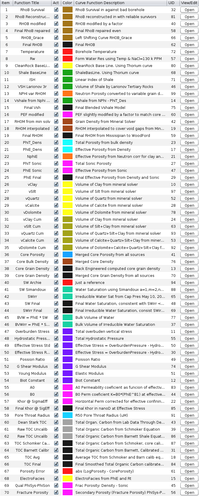
• A tight reservoir with a carbonate mineral solver and shale oil.
  
  ✔ GLOG File: shaleOil.glog
  
  This example shows a typical work-flow to process a tight reservoir with a mineral solver for clay and carbonate minerals. Also the deeper zone has a shale oil play for which TOC Total Organic Carbon is computed using the Schmoker equation calibrated with laboratory pyrolysis data. The track Minerals shows a reasonable agreement between mineral proportions estimated by lab XRD X-Ray Diffraction, and GeolOil mineral solver ↓

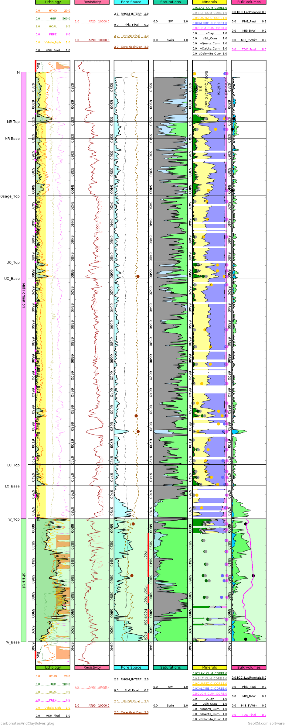
The sequential functions panel work-flow below ↓ shows the steps that produce the interpretation.

---

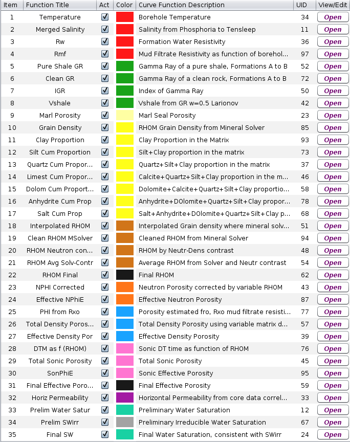
• A carbonate and eolian reservoir with mineral solver and estimation of matrix density.
  
  ✔ GLOG File: RHOM1_WebExample.glog
  
  An accurate estimation of the matrix density RHOM ρ_m is a fundamental task for any petrophysicist. In complex reservoirs ρ_m is no longer an approximate constant value inferred from the depositional environment, but significantly varies with depth. That is ρ_m = ρ_m(depth). Once RHOM is estimated, it is used to compute porosity and water saturation —and also to estimate permeability— The brown rightmost last track "RHO matrix" on the log plot below shows how to estimate the matrix density RHOM ρ_m using only well log curves, without any core lab measurements available ↓

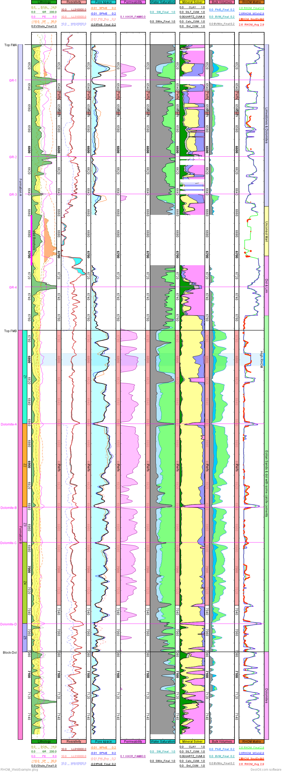
The sequential functions panel work-flow below shows the steps that produce the interpretation.

---

• A clean eolian reservoir with indicator curve flags for net-sand and net-pay
  
  ✔ GLOG File: wellExampleNetPay.glog
  
  The example below ↓ shows a log plot with indicator curve flags (GeolOil exclusive trilean logic: -1 for no, +1 for yes, 0 for inconclusive) for net-sand and net-pay. After computing cutoffs for porosity and water saturation —this eolian rock is very clean, so computation of Vshale cutoff is waved: GR here does not read clay, but remnants of organic bio-radioactivity and signal noise—, the indicator flag curves are produced with the Filtering & Upscaling module.

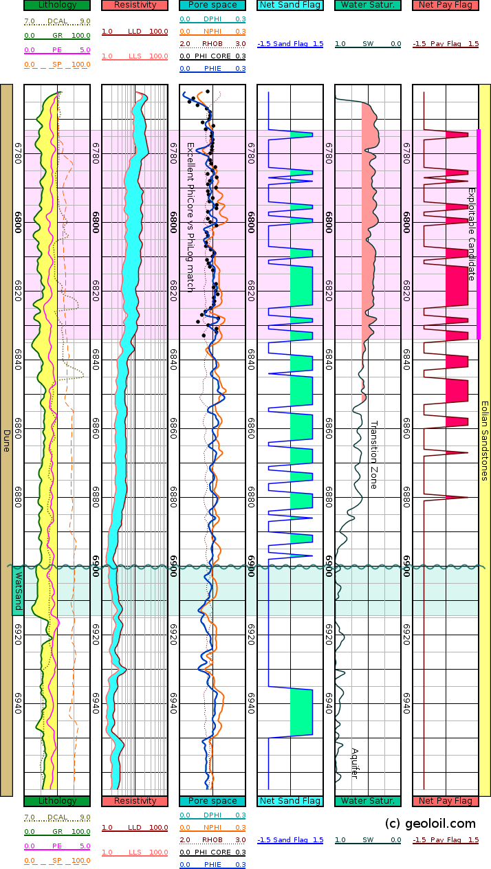
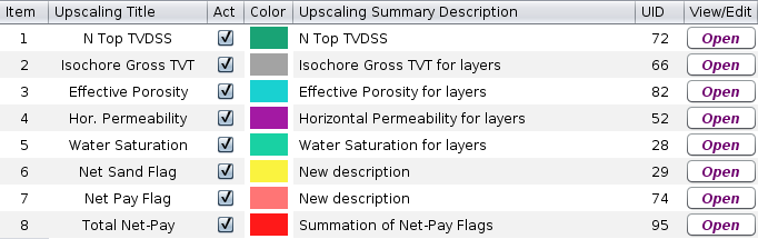
The Upscalings Panel work-flow below ↓ shows the steps that produce the indicator curves

---

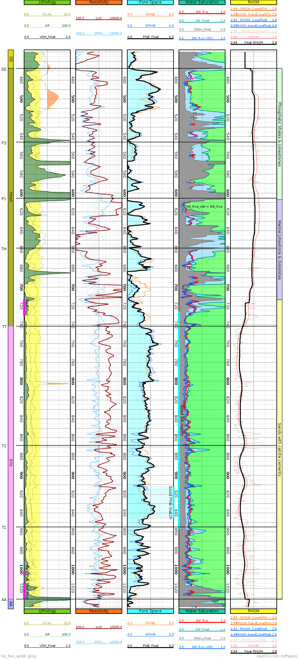
• An eolian reservoir with water saturation computed through the SW ratio method without porosity
  
  ✔ GLOG File: Sw_Rxo_wellB.glog
  
  The example below ↓ shows in the fourth track, the water saturation computed by the technique of the SW ratio flushed zone method without using porosity (the red curve), and its comparison the water saturation computed by the Indonesia equation that uses porosity (the aqua-marine curve). The agreement between those curves is good, especially where the rock is less clayey.

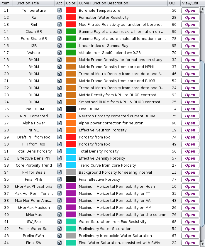
The sequential functions panel work-flow below ↓ shows a snippet of the steps that produce the interpretation.

---

• A gas reservoir with porosity computed through five different techniques
  
  ✔ GLOG File: Phi_Rxo_and_Gas_DTF.glog
  
  The example below ↓ compares on the third track, five porosity computations from different methods: porosity from micro-resistivity, density porosity, neutron porosity, sonic porosity, and core porosity. Notice that the sampled core plugs seemed to be expanded at surface, increasing slightly the correct in-situ porosity.

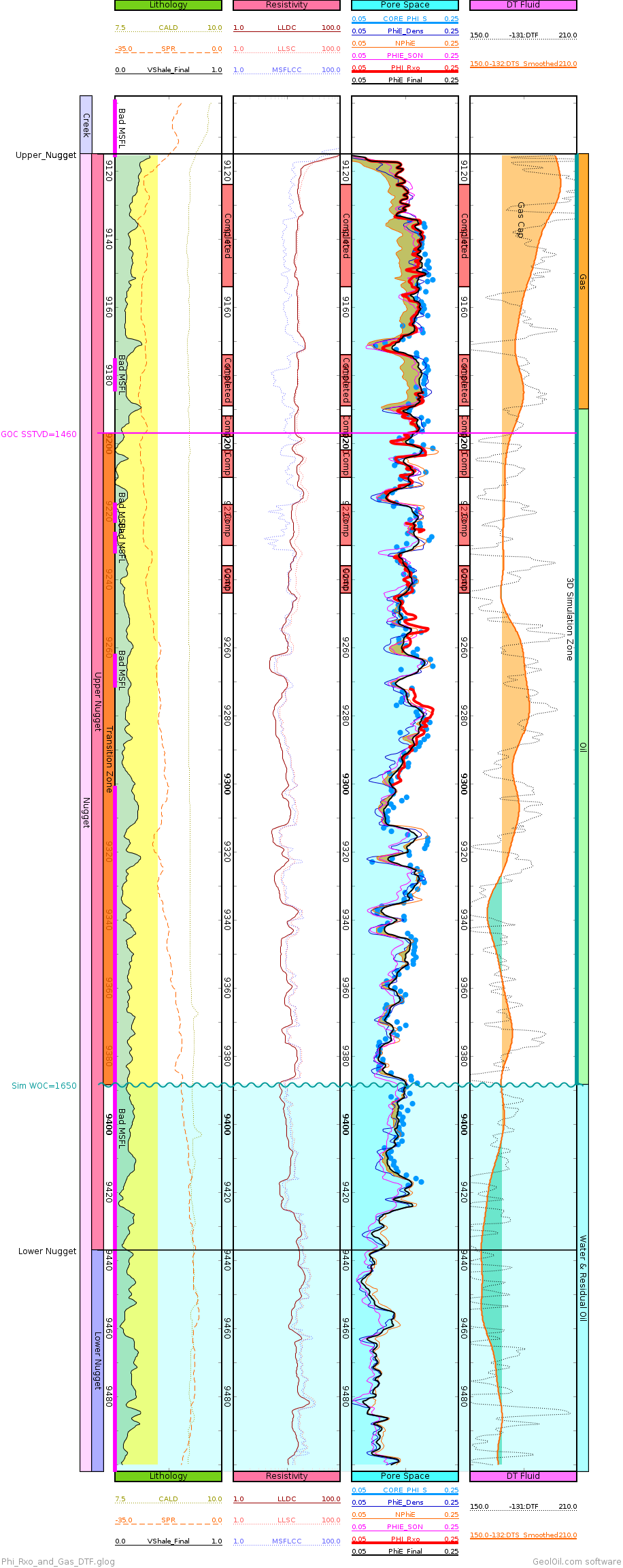
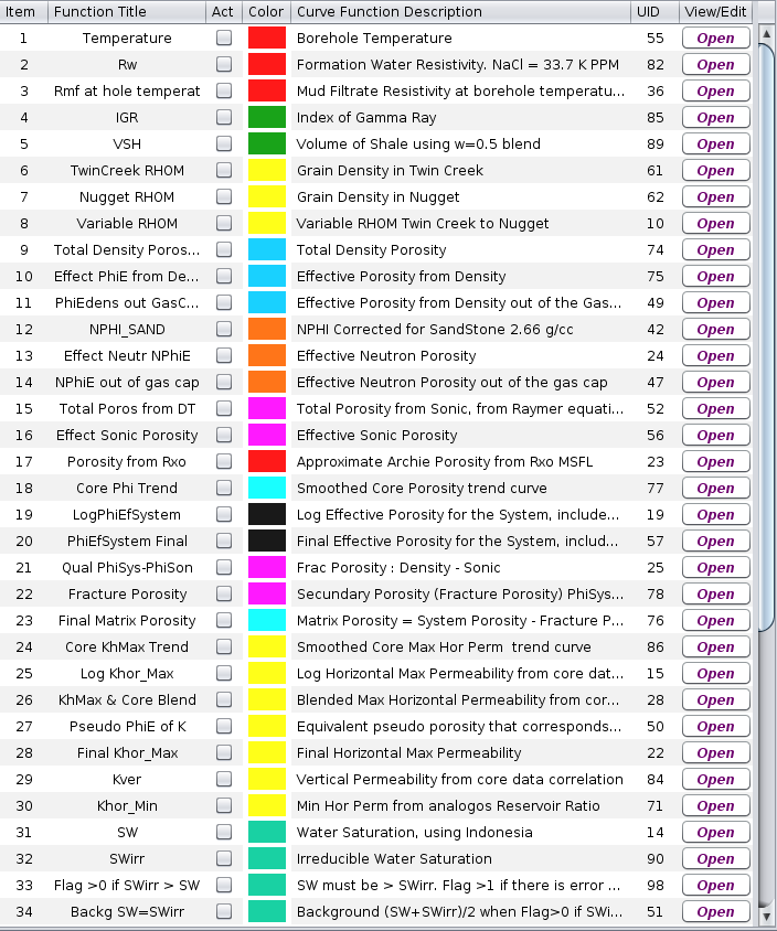
The sequential functions panel work-flow below ↓ shows a snippet of the steps that produce the interpretation.

Related article: How to access the default GeolOil built-in minimal data set of examples

GeolOil is listed by the official SPWLA software directory

© 2012-2025 GeolOil LLC. Please link or refer us under Creative Commons License CC-by-ND