


 TRAINING


 PAPERS
 REFERENCES
 GET IN TOUCH

|

|
 Downloads
|
 Prices
|
 Videos
|


|
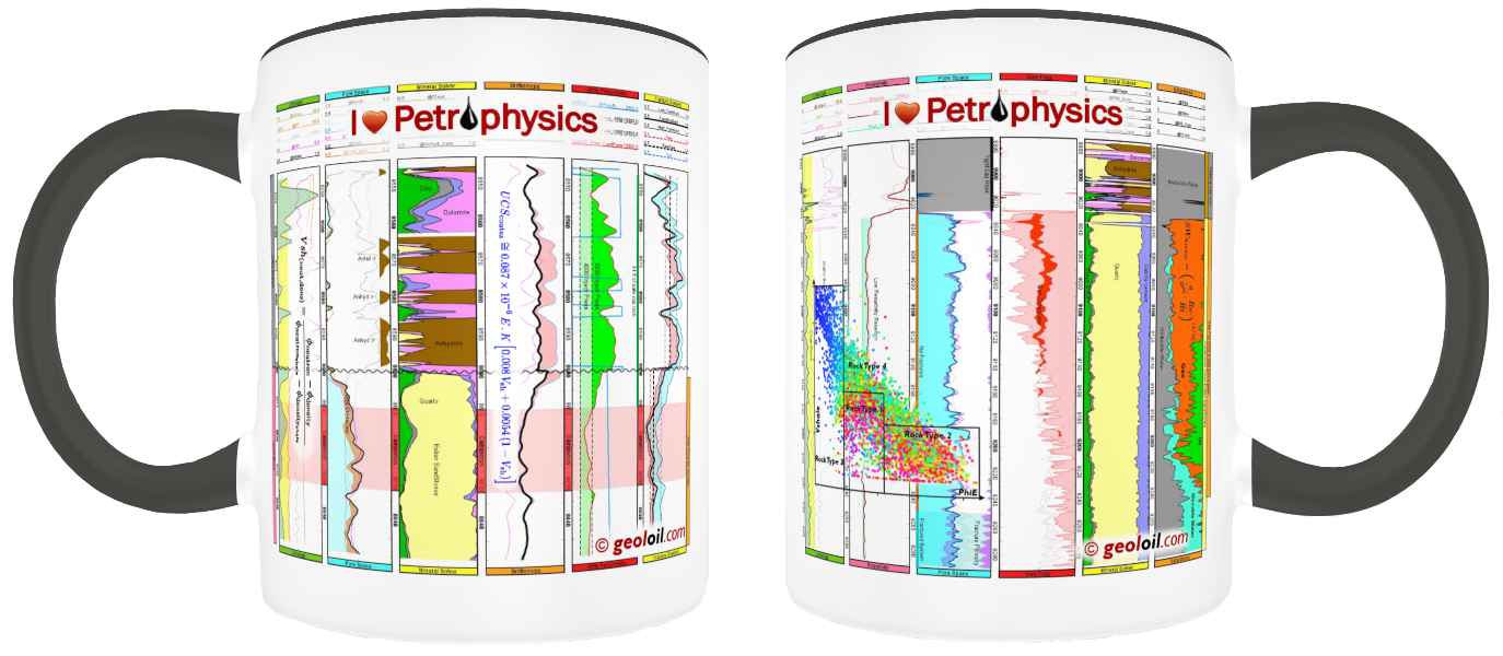
"I love Petrophysics" |
GeolOil - How to calculate Shale Volume from Gamma Ray: Larionov, Clavier and Stieber models
 This is one of our most referenced articles on the internet
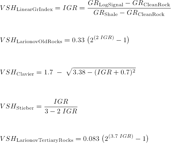
Estimating the rock's shale volume VSH linearly from the gamma ray log still remains the first preferred approach to become with a preliminary shaliness indicator. The procedure is easy and straightforward, and might give reasonable results for some deep reservoirs. The first equation shown below defines an IGR shaliness index as a function of the GR gamma ray log signal: It only needs to record the response of the gamma ray log for a nearby known shale body and a nearby known clean rock.
However, quite often the linear IGR shaliness indicator yields an over-estimation of rock's volume of shale (specially for shallow, young reservoirs), producing an overall pessimistic scenario of the reservoir quality. To overcome this, several empirical formulations have been developed to correct and reduce the rock's shale volume Vshale as direct functions of IGR, that is VSH = f (IGR), trying to adjust the clay minerals total radioactive response.
Ordered from the most pessimistic shale indicator IGR (more VSH), to the most optimistic one, the Larionov VSH equation for young, tertiary rocks (less VSH), the equations show the Linear VSH IGR indicator, the Larionov model for older rocks, the Clavier model, the Stieber model, and the Larionov model for tertiary rocks:
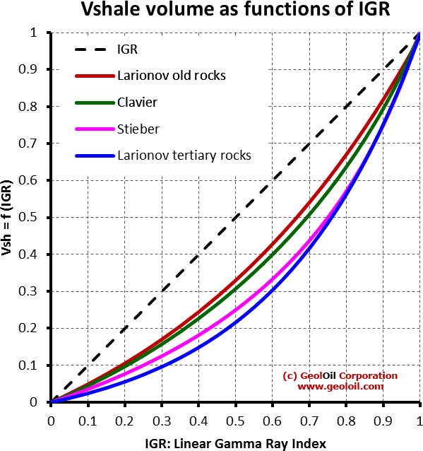
Different vshale corrections VSH = f (IGR), as functions of the IGR index. The corrections are particularly important for medium IGR values around 0.4 - 0.7:
Why handle completely different equations? One workaround is compute only the extremes: pessimistic linear IGR (more Vshale), and the optimistic Larionov for tertiary rocks (less Vshale) to derive a custom blended combination:
VSH_geoloil (IGR, blend) = blend*IGR + (1-blend)*VSH_larionovTertiary
where blend is a parameter in the range [0,1]. The closer to 1.0, the more weight is given to IGR (more Vshale), the closer to 0.0, less weight is given to IGR (i.e. less Vshale: a cleaner rock). A yet simpler workaround is to use a common generalization of the Stieber equation:
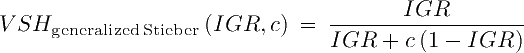
This generalized Stieber equation, reduces exactly to the regular Stieber equation when c=3, replicates exactly IGR when c=1, and yields VSH=0 as c → ∞. If c ≥ 1 is handled as a continuous parameter —instead of typically suggested fixed integer values 3, 2, and 1—, the equation is versatile enough to provide good approximations to the empirical models of Old-Larionov, Clavier, regular Stieber, and Larionov for tertiary rocks. Just find a suitable value of c by minimizing the integrated squared difference error between the approximating function to its target function:

The choose of the weight function is not difficult. Chose an un-weighted constant w(IGR)=1 if a general overall accuracy is needed throughout the whole range 0 < IGR < 1. For practical reservoir exploitation optimization studies, we recommend to pursue a higher accuracy on pay rocks with lower Vshale by using w(IGR) = 1 - IGR.
| VSH model | un-weighted | w(IGR) = 1 - IGR |
| VSH = 1 | 0.00 | 0.00 |
| VSH = IGR | 1.00 | 1.00 |
| Larionov Old Rocks | 2.01 | 2.03 |
| Clavier | 2.27 | 2.27 |
| Regular Stieber | 3.00 | 3.00 |
| Larionov Tertiary Rocks | 3.33 | 3.48 |
| VSH = 0 | ∞ | ∞ |
Values of c required to produce good approximation functions to the Vshale models
How to choose a value for c if there is not lab data for a calibration or select a VSH model?, there is nor a closed or easy answer. The petrophysicist or geologist interpreter might pick a value from his/her judgement, experience, nature of the reservoir, and available XRD lab data for calibrations. The interpreter may compute also different estimates of VSH that don't depend upon the gamma ray log to guide the decision, like the neutron porosity to density porosity difference technique:

The former equation can be applied over different formations, members, beds, and facies, to compute the optimum c parameter per zone. It can be seen as some form of supervised learning, using only commonly available log data, without using X-Ray diffraction XRD lab data for further calibrations. Once a collection of c parameters is estimated, a variable non-constant log curve can be used to compute a VSH(z) curve without switching Vshale model equations per zone.
Below we show a well-log from a case study for a shallow Wyoming reservoir. In this particular case, the linear IGR index yielded a clearly pessimistic, over-estimation of rock's shale content:
The blue "Zone 2" on the GeolOil log plot panel below, shows a pay zone with a deep resistivity around 30-40 Ohm.m. The magenta "Zone 1" on the top log's plot panel shows a resistivity of around 30 ohm.m. According to the linear IGR VSH, the zone 1 shaliness (dashed red curve) is more 0.50 V/V units. It is quite difficult to believe that such high resistivity zone, could come from a very shaly sand body. Both the Larionov tertiary rock VSH estimate and the VSH estimate from the Neutron Porosity to Density Porosity distance yield more reasonable lower VSHALE values around 0.25 - 0.30 V/V, allowing hydrocarbon accumulations.
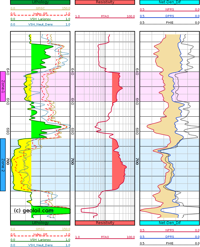
Comparing three VSH estimates in the first track: the Linear IGR index (dash red), Larionov (solid green) and Neutron-Density difference (dotted blue).

Panel with different equations to estimate VShale.

|
Related articles:
|
|
| |


|
|
|
© 2012-2026 GeolOil LLC. Please link or refer us under Creative Commons License CC-by-ND |