


 TRAINING


 PAPERS
 REFERENCES
 GET IN TOUCH

|

|
 Downloads
|
 Prices
|
 Videos
|


|
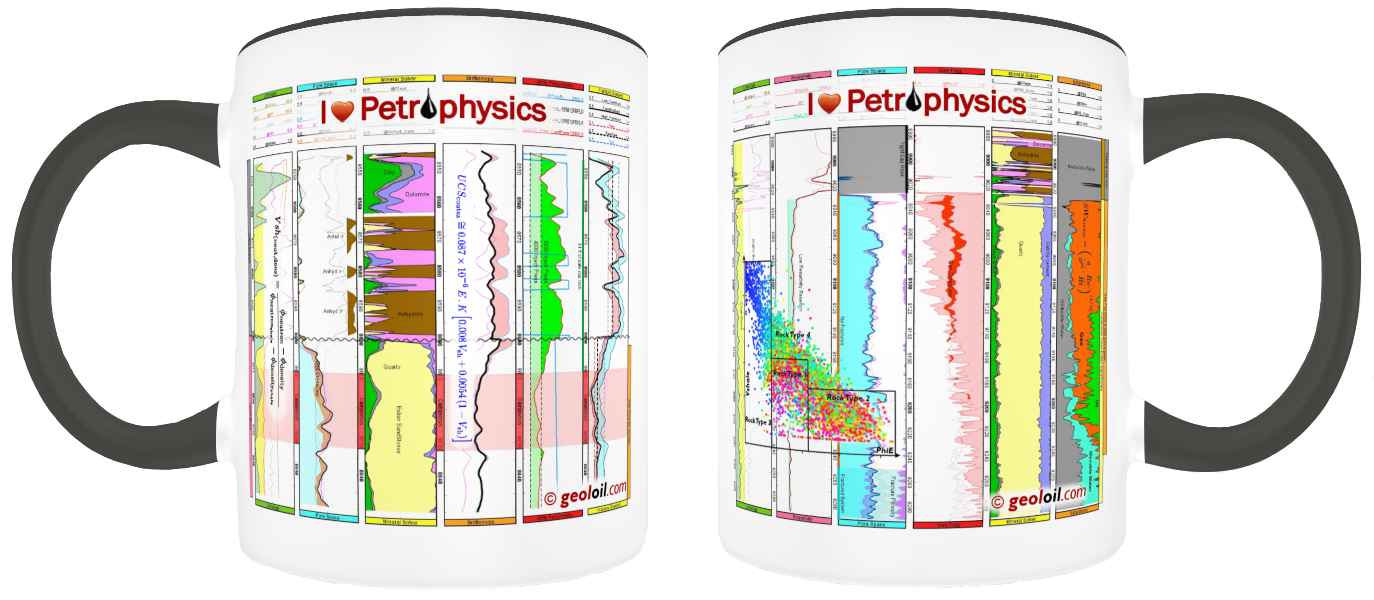
"I love Petrophysics" |
GeolOil - How to Calibrate Well Log Curves
Curve calibration is the process that transforms an original curve signal y=f(x) from "unreliable" or undesired magnitudes to a "more correct" or better suited t=g(x) values that fits a purpose. It includes changes to the original signal range to a desired range output, and corrections to the curve. A mapping calibration function cal(•) is a strict monotonic function applied to the original curve signal points {yi}i=1,2,...,n that produces a final transformed signal {ti}. That is, t = cal (f(x)). Since cal(•) is an invertible function, there is no loss of information as the signal y can be restored by y = cal-1(t).
GeolOil techniques to calibrate a Vshale well log curve
This article first published on Dec 4th 2022, introduces the GeolOil Soft-Ceiling calibration technique for positive physical properties —with the notable exception of SP Spontaneous Potential, almost all petrophysical properties like porosity, volume of clay, permeability, and water saturation, have positive values and a bounded, limited physical maximum—
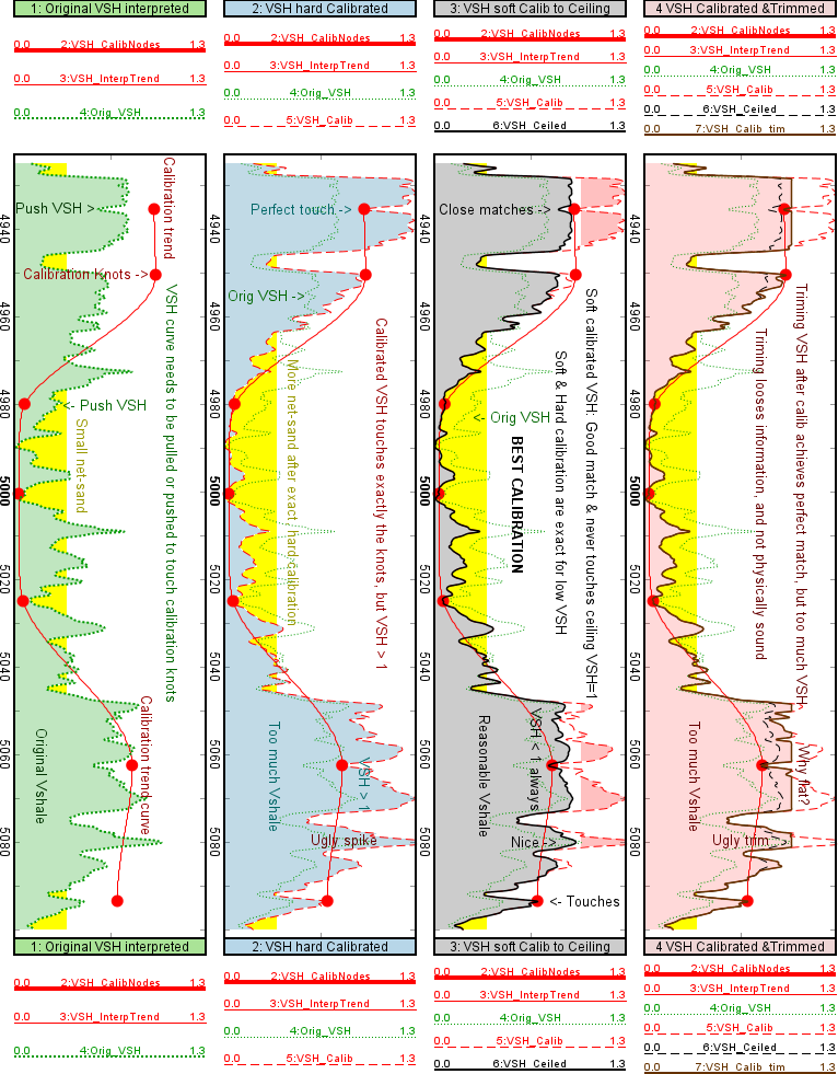
The image above shows in the green first track, an original Vshale curve VSH=f(depth) with accuracy issues. The depths above MD=4,960 ft have lower than expected VSH values. This zone is known to be a sealing cap rock. The correct values of VSH at the red knot depths of 4,935.5 ft and 4,950.5 are thought to have shale volumes of around 95% and 96%. The zone from depths 4,980 to 5,025 ft have higher that expected VSH values, the zone is known to have very clean rocks with VSH 3%-5%.
The green original poor VSH curve needs to be calibrated with a process that satisfies the five GeolOil Soft-ceiling calibration principles:
- Honors 0.0 values exactly —the calibration is anchored at zero— As a counter example, arithmetic shifting (to add or subtract a constant) can't honor an original value of zero.
- Does not yield negative values. As a counter example, arithmetic left shifting can easily yields negative values.
- Passes as close as possible to knot calibration points, and follows a specified trend calibration curve.
- Preserves the general qualitative shape of the original curve. As a counter-example, no trimming procedure complies with this: it ends assigning a slope of zero for values that exceeds the maximum, thus loosing all information of non-zero slope zones.
- Never exceeds the physical maximum or "ceiling" (even if the original curve exceeds the maximum). As a counter-example, arithmetic shifting, proportional transforms, and linear transforms easily exceed allowed physical limits.
The gray third track shows a GeolOil Soft-ceiling correctly calibrated VSH curve that preserves the general shape and yields 0 ≤ VSH ≤1. It honors all the five calibration principles.
The blue second track shows a depth adaptive proportional transform that fails on its attempt to calibrate VSH: although it succeeds to pass exactly over all the red calibration knots and follow the trend curve, it completely fails to honor the physical maximum of VSH, that should never exceed 100%. The last pink track is essentially the same as the blue second one, but trims or limits VSH values greater than 100%, yielding an artifact, non-realistic flat behaviour that completely looses all information for very shaly rocks. Both the blue proportional transform, and the pink trimmed curves fail to shrink VSH values for high magnitudes. Hence producing quite large volume of shale over-estimations.
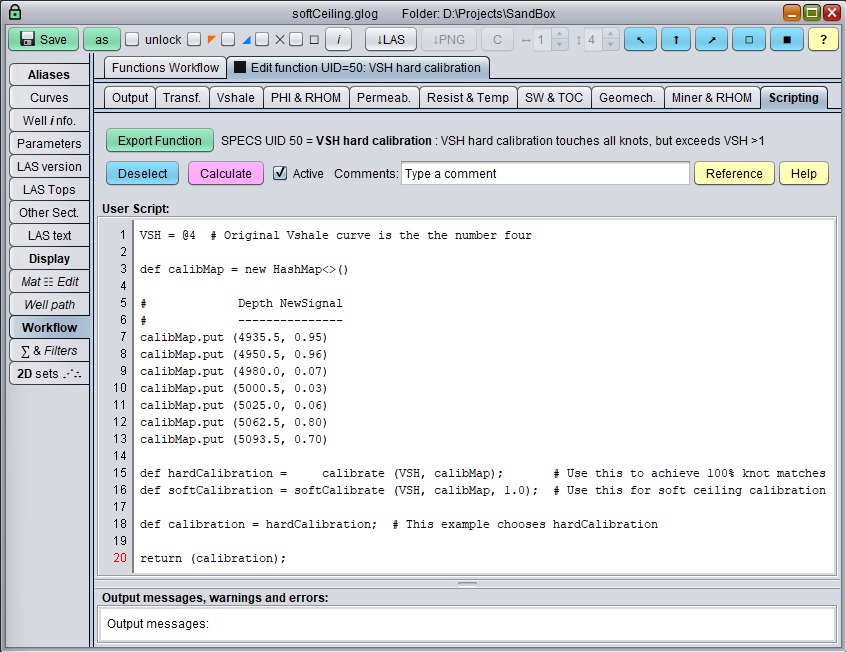
Script to calibrate curves using a proportional transform. Choose softCalibrate() to use the GeolOil Soft-ceiling calibration instead
Instead of typing the above minimalistic short script to apply the GeolOil soft-ceiling algorithm, you may prefer to use a GUI window, like the one shown below. First compute a "hard calibration" of the original curve, and then dynamically compress the curve to asymptotically reach its maximum physical value or "ceiling". By "soft" we mean that the maximum is only reached for very large signal values, but it is never exactly touched —in math, the maximum ceiling is called the "supreme"—
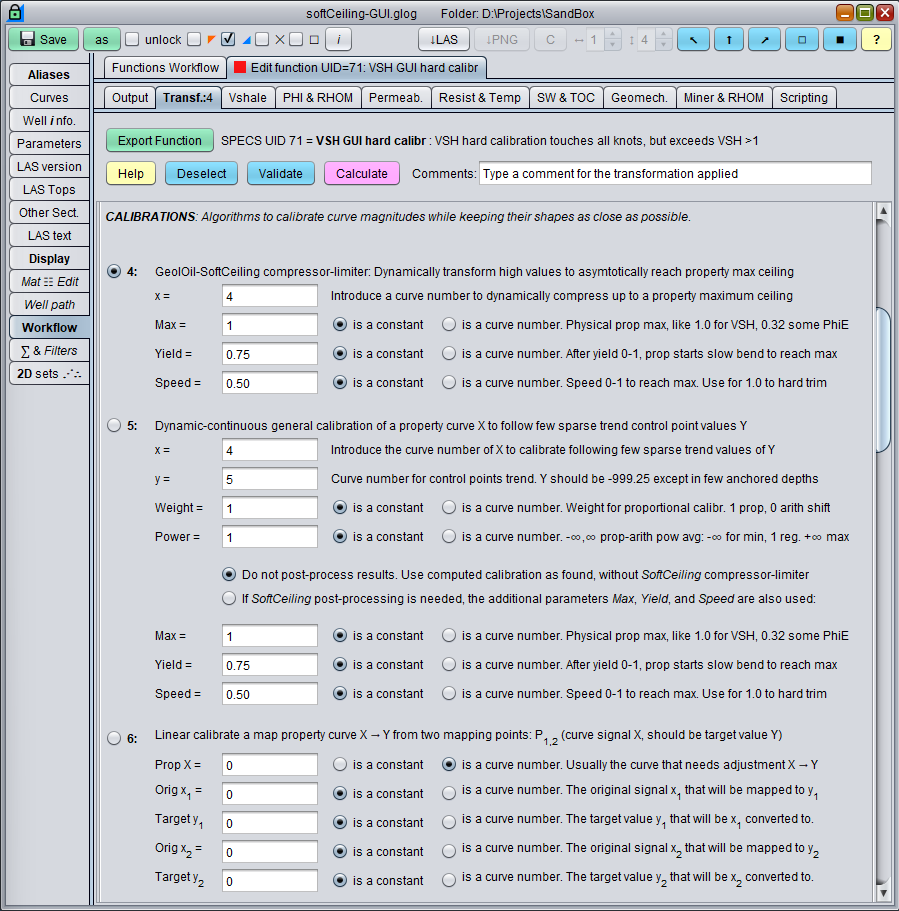
GeolOil GUI panel for Soft-Ceiling well log curves
There are three parameters to specify for the adaptive soft-ceiling dynamic compressor:
- The Maximum is the expected allowed property ceiling. The user must explicitly type its value, don't rely on the default value of 1.0. For instance, it is 1.0 v/v for volume of shale, volume of clay, mineral proportion solvers, and fluid saturations. For unconsolidated loose sands, effective porosity PhiE may be around 0.32 v/v, and for tight carbonates could be around 0.15 v/v. Likewise, absolute permeabilities ceilings for unconsolidated sands may be around 10,000 milli-Darcies, and around 10 milli-Darcies for some tight carbonates. But shale oil plays could be in the range of nano-Darcies.
- The Yield point (0<yield<1), is the proportion of the maximum where the curve starts its gentle soft bending to asymptotically reach its maximum. Before the yield point (0 < hard calibrated signal/maximum < yield), the output is essentially a clone of the input value. Yield values around 0.70-0.80 usually give good results. The yield parameter is similar to the concept of downward threshold compression in the context of dynamic range sound compression engineering.
- The Speed parameter (0<speed<1) specifies how quickly the algorithm tries to reach the ceiling. A value of 1.0 is equivalent to a regular hard trimming that clips the signal to its maximum once the input curve reaches the declared maximum —a non-asymptotic behaviour— After the maximum, the output stays flat to this maximum. Such speed of 1.0 results in a similar behaviour called "hard knee " in the context of sound compression theory. The default value of 0.5 usually gives good results, with a smooth behaviour and continuous 1st and 2nd derivatives of the cal(•) calibration function. Use a speed of 0.0 to very slowly reach the ceiling asymptotically.

|
Related article:
|
|
| |


|
|
|
© 2012-2026 GeolOil LLC. Please link or refer us under Creative Commons License CC-by-ND |