How to calculate Net-Sand and Net-Pay

Calculating reservoir net-sand and net-pay values are standard tasks on many geology and petrophysics projects. While the concepts involved behind the calculation are simple, there are some fine details on how to make a precise or custom evaluation. Many experienced geologists can approximate a value for net-sand and net-pay by just looking to the log's gamma ray and deep resistivity curves for simple reservoirs. However, there are complex reservoirs for which a visual evaluation is neither enough nor accurate. Here GeolOil comes to help, allowing to compute net-sand and net-pay with big versatility in six steps:

The first step to compute net reservoir rock, net-sand, or net-pay for a given zone is to ensure that the well geometry has been properly defined. If the well is slanted or non-vertical, a direct count or visual inspection to its log measured depth MD, will yield an overestimation of the real net value. In these cases, the well's directional or deviation survey file has to be loaded, and it must have at least the minimum set of four columns: MD, TVD, DX and DY. With this information, GeolOil will calculate all the necesary verticalized depth step intervals.

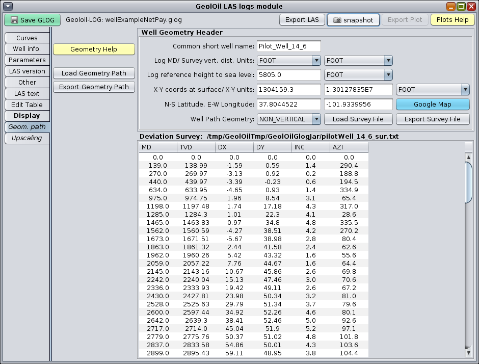
The figure below ↓ shows a well's header geometry path loaded in GeolOil

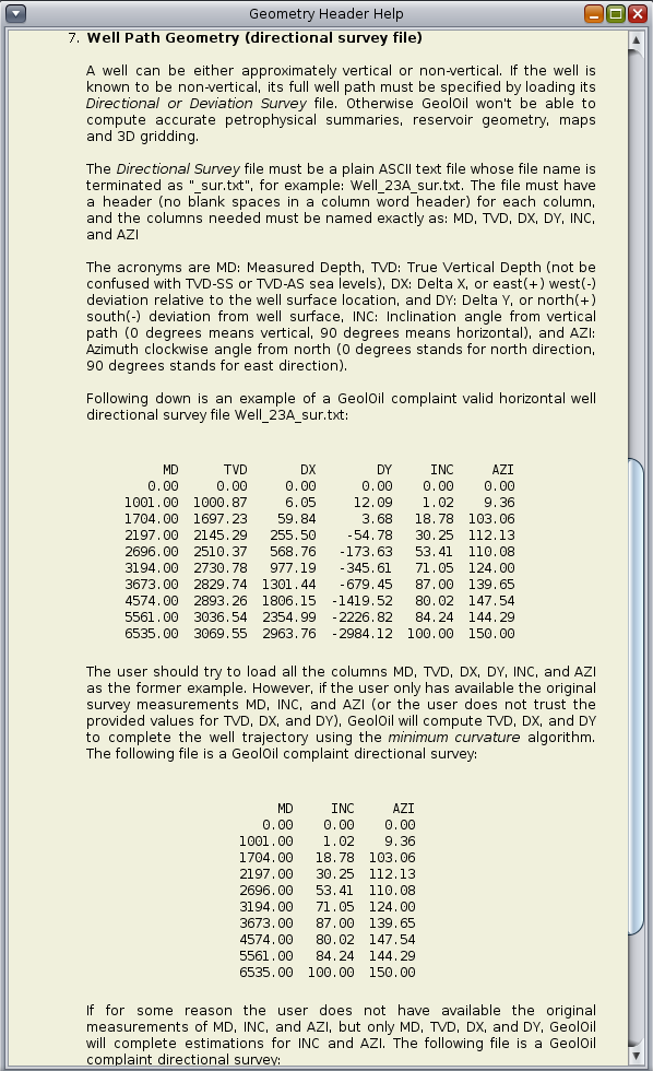
The figure below ↓ shows a piece of GeolOil help to load a Deviation Survey file

Once the well's geometry directional survey path has been loaded, the user can declare a list with the intended upscalings to be computed. In GeolOil, net reservoir rock, net-sand, and net-pay are considered as indicator extensive upscalings. In a typical project, the upscaling list should contain entries to compute not only net-sand and net-pay, but also to calculate the upscaled porosity in reservoir rocks and pay rocks, as well as some sensibilities to define petrophysical cutoffs.

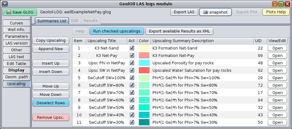
The figure below ↓ shows the upscaling list panel. Notice that net-sand, net-pay, porosity and water saturation were included.

In the second step, the user opens the row for net-sand, and declare the processing type as "extensive upscaling". Properties like summations, net totals should be treated as extensive properties.

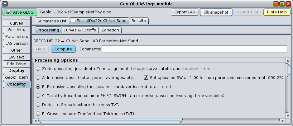
The figure below ↓ shows the Processing Panel, with extensive upscaling selected.

The third step is to define the cutoff system for the reservoir under study. The user usually enters here values from a former legacy study. However, GeolOil encourages the user to validate, update and estimate the petrophysical cutoffs using our recipe. A cut-off system is a set of petrophysical filters that are applied to a rock to detect its matching lithotype target. For each particular case of computing net-rock or net-sand for a fluid bearer reservoir rock, the user needs to specify what values of shaliness and effective porosity bear movable reservoir fluids, including water, oil, and gas. (net-pay should only consider movable, producible, or exploitable oil or gas hydrocarbons)

There are no fixed rules on what petrophysical properties should be filtered. In many clastic reservoirs, cutoffs are applied to detect clean sandstone porous rocks. Hence cutoffs like Vsh < 30% (for which gamma ray could be around GR < 65 API units in some reservoirs), and effective porosities around PHIE > 7% are found quite often. Other clastic reservoirs can have dolomitic sands embedded, so it will advisable to apply a filter for photoelectric factor that discards dolomite minerals with a PEF value of around 3 Barns/E. That is, using a filter like: 1.7 < PEF < 2.2 will accept only quartz sandstones.

Other sedimentary environments, like some marine limestones carbonate reservoirs and some eolian sandstone reservoirs almost don't have clay minerals in the rock's fabric. In those cases, GR is usually very low, bringing a base line of white noise that could be discarded. On other cases, the radioactivity response is not associated at all with clay minerals, like in radioactive sands.

The case study illustrated in this article, is a clean eolian sandstone reservoir. After a very low estimation of Vshale was calculated, it was decided not to apply any filtering for shaliness, and if some Vshale filtering would have been applied, the rock would easily passed the filter. In the image below, notice that item row number three specifies the porosity curve at the position 14 of the LAS file (the user can always edit the LAS file mnemonic list with GeolOil and move the curves to any desired position). Also notice that the item row number zero, declares no "target property" (curve number is 0). This tells GeolOil that no property will be introduced in the pore space, so the extensive upscaling will consist to apply the cutoffs to the rocks, raise an indicator flag for each verticalized depth step and calculate a depth summation to yield a net-sand summary value.

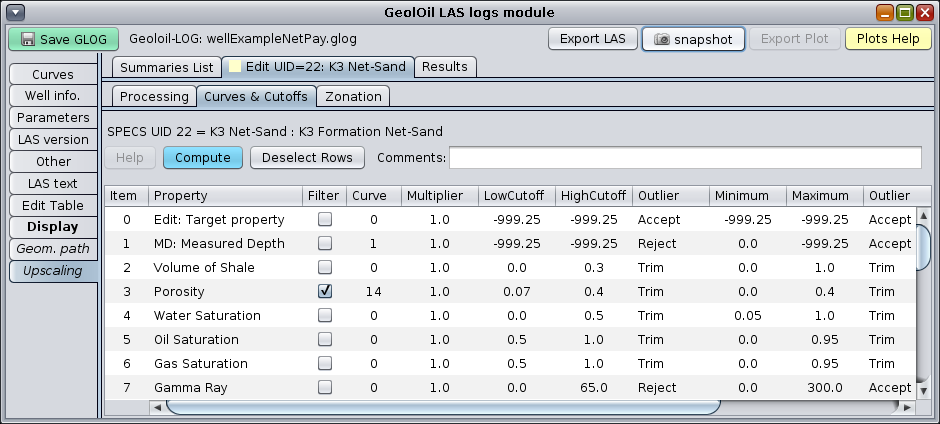
The figure below ↓ shows the cutoffs panel, where only rocks with porosities of more than 7% are accepted.

The fourth step is to declare for which zones the upscaling will be computed and specify an output indicator flag curve for net reservoir rocks. The case presented asks to compute upscaling for "Formation" zones (and particularly the zone ID=71). The output indicator flag curve was named with the mnemonic "NetSand".

The figure below ↓ shows the "Zonation Panel" to select the stratigraphic zones and specify curve outputs.

This step involves the same concepts and considerations discussed for net-pay, but with one difference: the rock must bear significative oil or gas hydrocarbons in its pore space. This means that an additional petrophysical property must be specified: that property is water saturation. In the image below, the water saturation curve is found in the position 20 of the LAS well log, and its cutoff filtering was 0 < SW < 60%.

However, what can be done if the user has to do a quick and dirty flash study of a reservoir with raw, non interpreted original curves?. In such cases, some simple reservoirs can be screened with an approximate quick cutoff system. We have seen some clastic reservoirs to respond reasonably well with only two cutoffs of around GR < 60 API units, and a deep induction resistivity cutoff (this value would depend upon reservoir temperature and formation water salinity, so there is no a default or standard value to be referred or suggested, even approximated).

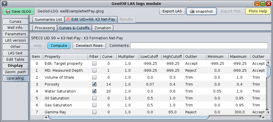
The figure below ↓ shows a cutoff system for net-pay. It's the same as net-sand, but SW is added.

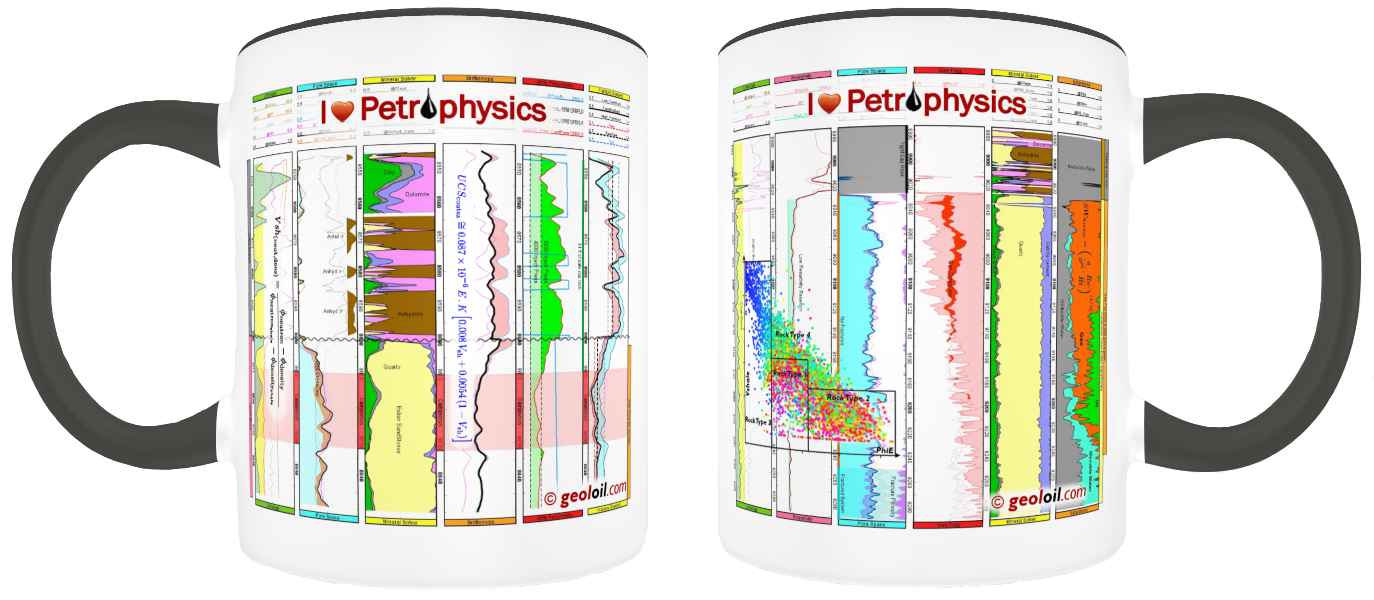
Finally the user can plot the resulting curves. In the image below, the Net-Sand track shows the reservoir rock indicator flag corresponding to net-sand with fillings in aqua color. The Net-Pay track shows the pay rock indicator flag with fillings in burgundy red.

✔ NOTE: The GLOG file work-flow for this log is available for download with the set of optional interpretation examples.

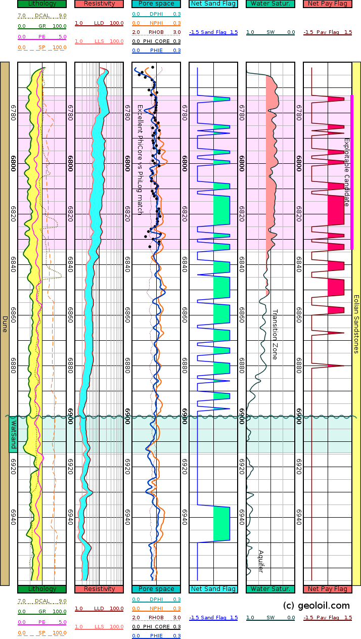
The figure below ↓ shows a plot of indicator flag curves for net-sand and net-pay.

Related articles: How to compute Petrophysical Cutoffs How to estimate VSH from Gamma Ray How to estimate VSH from Neutron-Density porosity difference

Related video: How to compute net-sand, net-pay, and property upscalings